May 26, 2025
in Dashboards
We have added a new window option to the dashboard; Total Return Chart.
The new chart displays the total return value of 1 or 2 securities over the specified lookback period.
The dashboard example below has 4 charts that show the performance of EFA and SPY over 3, 6, 9 and 12-months.
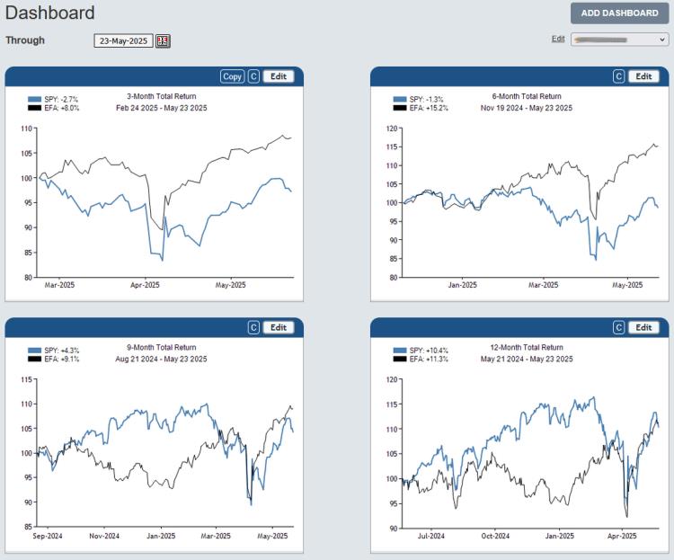
click image to view full size version
See: Introducing Dashboards: A Way To Help Organize Workflow In Research & ETF Portfolio Backtesting
Apr 08, 2025
in Channel, Parameter Summary
We have made two upgrades to the Channel Parameter Performance Summary.
Firstly, the Channel Parameter Summary now allows a range of Buy and Sell points to be tested. Whereas previously only a single Buy and Sell point could be specified, it is now possible to set min, max and step values for these two parameters.
Secondly, a Substitute function has been added, which allows a different / replacement security to be specified for the execution of the actual trades. For example, a channel can be based on the Total Return value of QQQ, but the resulting trades can be executed in QLD.
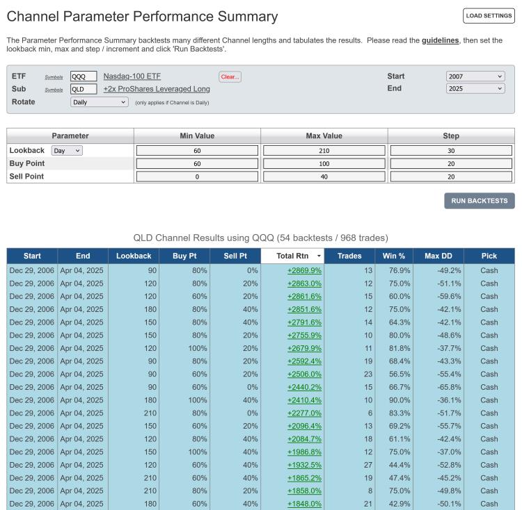
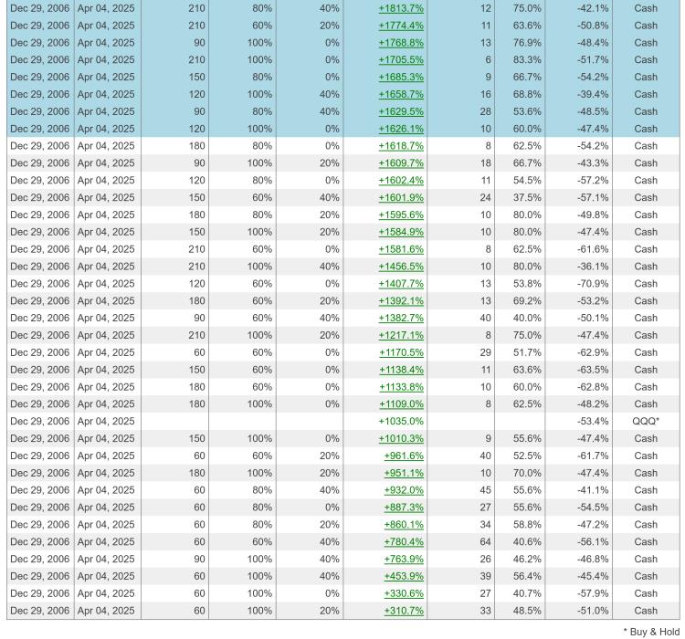
click images to view full size versions
Go to the Channel Parameter Performance Summary
Notes:
- Studying the guidelines is strongly recommended.
- Parameter Performance Summaries are available to both regular and pro annual subscribers
Mar 04, 2025
in Moving Average, Channel
We have added a 'Substitute' function to the ETF Moving Average and Channel backtests.
Clicking 'Substitute' allows subscribers to specify a different / replacement security for the actual trades. For instance, in the example below the backtest invests in QQQ when XLK is above its 12-month Exponential Moving Average (EMA).

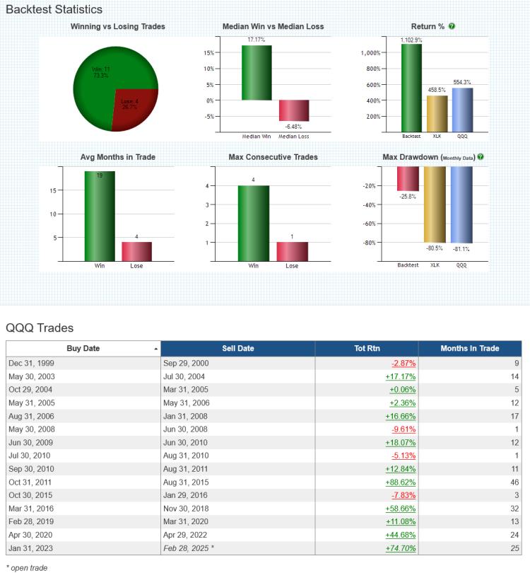
click chart images to view full size versions
The Substitute function is available to all subscribers on the following backtests:
Note:
To test investing in Portfolio A when x security is above its MA and Portfolio B when x security is below its MA, use the Regime Portfolios backtest.
Feb 14, 2025
in Regime Change
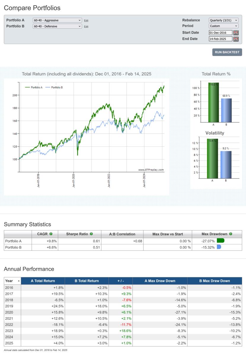
In 2016 we wrote a blog post with an example that employed a simple credit spread style ratio (HYG / IEI) as a regime indicator to switch between aggressive and defensive 60- 40 allocations.
When the High Yield / Treasury ratio was in an up trend (i.e. HYG / IEI was above its 6-month moving average) the backtest invested in the aggressive portfolio, which contained Emerging Markets, Financials, Nasdaq and High Yield ETFs. When the ratio was below its MA, the backtest switched to the defensive 60-40 portfolio that held Treasury Bonds, Utilities, Healthcare and Consumer Staples.
Below is an update of the same Regime Portfolios backtest, starting from the end date of that blog post example; December 1st, 2016.
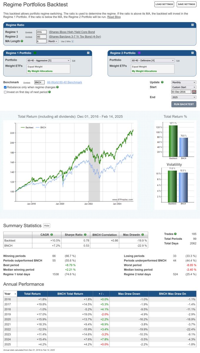
click chart image to view full size version
During the 9-year out-of-sample period since the original example, the regime model has been invested in the aggressive portfolio (Risk On) approximately 75% of the time. The performance of both the aggressive and defensive 60-40 portfolios, over the same time period, is displayed below.
click chart image to view full size version
As with the original blog post, this should not be viewed as a strategy to be replicated as is. Rather, its' purpose is simply to illustrate the regime change concept and to provide a starting point for subscribers to further develop with their own ideas.
See:
Regime Portfolios backest
Compare Portfolios backtest
Feb 05, 2025
in Regime Change, Sectors
The performance of different industrial groups will vary over the course of the business cycle. Consequently, it makes sense that sector allocations be revised when there is a change in the prevailing regime.
Below is an example that uses High Yield Bonds to define the market regime.1 When JNK is trending upwards (i.e. above its MA), the backtest invests in the following high Beta sectors; Financials (XLF), Industrials (XLI), Technology (XLK) and Consumer Discretionary (XLY). Conversely, when the JNK trends down (i.e. below its MA), the backtest switches to a portfolio of low volatility defensive sectors; Consumer Staples (XLP), Utilities (XLU) and Health Care (XLV). To keep things simple, both the high Beta and low volatility portfolios are equally weighted.2
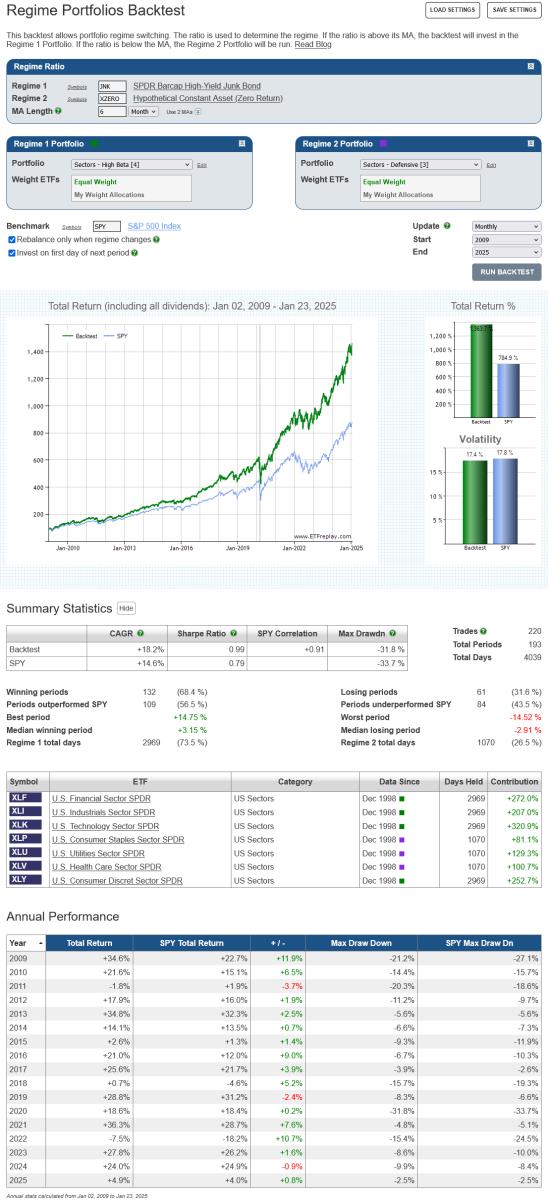
click image to view full size version
A simple alternative to choosing specific sectors from within an index (in this case the S&P 500), is to increase the leverage of the index itself when in Risk On mode or add cash when Risk Off. The following example employs the same High Yield regime, but this time the high Beta portfolio is 75% SPY and 25% SSO (2x daily S&P 500 return) and defensive portfolio is 75% SPY and 25% BIL.3
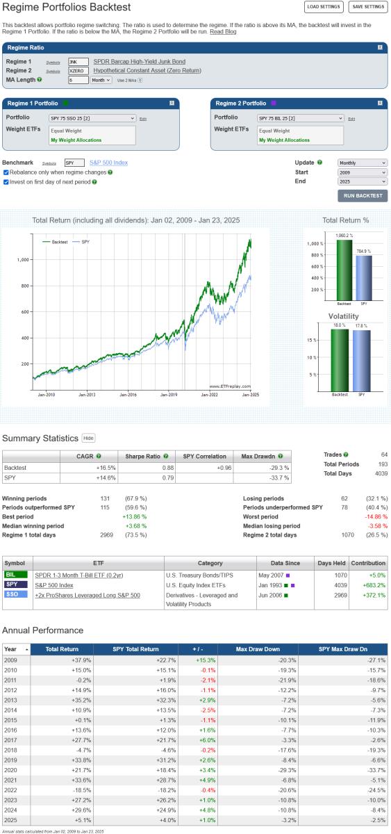
click image to view full size version
This simpler strategy produces far fewer trades. It should also be noted that as the high Beta and defensive portfolios are now just mildly levered / diluted versions of SPY, they will both be (almost) perfectly correlated with the S&P 500. While this could be considered a drawback, high-correlation to strong performing assets in up markets is consistent with Risk On strategy’s objective. The lack of diversification is less than ideal for the defensive portfolio, but the significant cash allocation will cushion losses in down markets.4
Notes:
- XZERO is simply a zero return index (i.e. it's a constant), so a 6-month MA of the ratio JNK / XZERO is the same as a 6-month moving average of JNK itself.
- An equal weight allocation will mean that sectors are over, or under, weight relative to their market capitalization weightings. Over the last 20+ years, the market cap value of the Health Care sector has been approximately 4 times that of Utilities. An allocation of XLP 35%, XLV 52% and XLU 13% would therefore be more in line with market capitalization weights.
- (75% * 1.0) + (25% * ~2.0) = ~1.25 Beta. (75% * 1.0) + (25% * ~0) = ~0.75 Beta
- Both examples employ a 6-month moving average to define the regime. When relying on any particular MA length there is always the risk that it will underperform in the future, even though it performed well in backtests. This risk can be attenuated by diversifying across a range of moving average lengths.